
The Parallel Decoding Trilemma
Published:
TL;DR: Parallel decoding is a fight to increase speed while maintaining fluency and diversity.
Recently, “Parallel Decoding” has become an active area of LLM research, especially with the proliferation of diffusion language models12345. The primary goal is to speed up LLM inference, but I think the tradeoffs involved are not fully understood by the community. I want to set the stage so that researchers understand this landscape and what will actually push the frontier.
I have written papers on this topic, specifically Accelerating Diffusion LLMs via Adaptive Parallel Decoding6 and Planned Diffusion7, and my opinions are heavily shaped by working on them.
What’s at Stake
Three properties are in tension:
- Speed — How fast can we generate?
- Fluency — How correct is the output?
- Diversity — How much coverage do we have over all correct outputs?
Speed
Let’s define these notions, starting with the most straightforward: speed. Speed (or latency) is simply the time it takes for an LLM to generate a response.
We can increase speed through parallel decoding: generating multiple tokens simultaneously. This is faster because it allows us to use fewer forward evaluations through the model to reach the final answer. In technical terms, we are reducing the depth of the computational graph required to produce the response.
In this blog, I’m going to focus on diffusion large language models (dLLMs) as a new paradigm to improve speed. That said, I believe my analysis of the tradeoffs between speed, fluency, and diversity extends beyond this specific paradigm and offers general lessons for LLM research.
Fluency and Diversity
Now let’s examine fluency and diversity together, as they are intrinsically linked.
- Fluency means the LLM generates “correct” things
- Diversity means the LLM provides good coverage over all correct things
When evaluating LLMs, people usually prioritize fluency and neglect diversity. This leads, for example, to LLMs that tell the same 25 jokes over and over 8 and contributes to an overall blandness of responses. I believe LLM generation diversity is underrated and critical, but I’ll address that more later.
Formal Definitions
Suppose there exists an ideal LLM distribution $p^*$. This $p^*$ is omniscient and god-like; its breadth of knowledge is immense, it can recall any fact, reason through any challenge, and can delight you in a multitude of ways even when given the exact same prompt repeatedly.
We are training a model $p$, and we can decompose the error between $p$ and $p^*$ using Total Variation Distance (TVD):
\[\text{TVD}(p, p^*) = \mathcal{L}_{\text{fluency}}(p, p^*) + \mathcal{L}_{\text{diversity}}(p, p^*)\]where we define the error components by integrating over regions where one distribution assigns greater probability than another:
\[\mathcal{L}_{\text{fluency}}(p, p^*) = \int_{\{x \mid p(x) > p^*(x)\}} \bigl(p(x) - p^*(x)\bigr) \, dx\] \[\mathcal{L}_{\text{diversity}}(p, p^*) = \int_{\{x \mid p^*(x) > p(x)\}} \bigl(p^*(x) - p(x)\bigr) \, dx\]These definitions mirror those in the paper Assessing Generative Models via Precision and Recall9. In fact, when $p$ and $p^*$ are Bernoulli distributions over binary outcomes, we recover the standard definitions of precision and recall. I rename these to fluency and diversity because they’re more apt for our context (and easier to remember).
Visualizing the Errors
This figure should make the concepts of diversity error and fluency error much more clear:
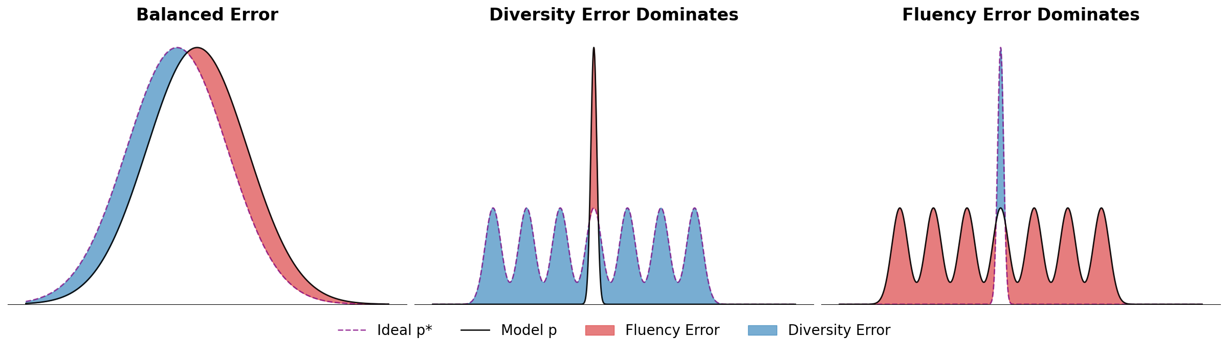 Three scenarios: balanced error (left), diversity error dominates when the model misses modes (center), and fluency error dominates when the model generates outside valid regions (right).
To summarize:
- If $p^*$ is multi-modal and $p$ only fits one mode → diversity error
- If $p$ generates data outside any mode of $p^*$ → fluency error
Fluency error is the type of error associated with “hallucinations”10. Diversity error will be associated with “mode collapse”11. Of course, this is a theoretical framework, and one never actually has access to the god-like $p^*$. These images are also a drastic oversimplication because LLM parameterize extremely high dimensional, multi-modal distributions that likely escape human intuition.
Diffusion Language Models (dLLMs)
Before discussing the tradeoffs between the above three properties, I must first explain diffusion language models. If you are already familiar with them, you may skip this section. Structurally, a dLLM is a BERT-style12 architecture. It takes tokens as input—some of which are [MASK] tokens—and predicts what should fill those masked positions. Diffusion language models predict the marginal probabilities over the [MASK] tokens given the existing tokens.
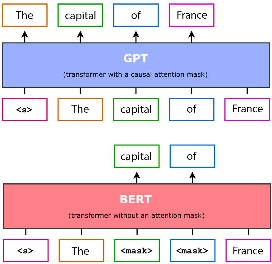
Here is a table summary of the differences between diffusion and autoregressive models:
| Autoregressive | Diffusion | |
|---|---|---|
| Architecture | GPT | BERT |
| Masking | Causal Attention Masking | Masked Token Input |
| Training | Exact NLL | Denoising ELBO |
| Inference | Sequential | Parallel |
Formally, consider a data point as a sequence of $n$ tokens $x = (x_1, \ldots, x_n)$. For sets of indices $\mathcal{Q}, \mathcal{O} \subseteq {1,\ldots,n}$ where $\mathcal{Q} \cap \mathcal{O} = \emptyset$, a masked diffusion language model $p_{\text{D}}(\cdot \mid \cdot; \theta)$ computes the marginal probabilities of tokens with query indices $\mathcal{Q}$ conditioned on tokens with observed indices $\mathcal{O}$:
\[p_{\text{D}}(x_\mathcal{Q} \mid x_\mathcal{O}; \theta) = \prod_{i \in \mathcal{Q}} p_\theta(x_i \mid x_\mathcal{O})\]where $p_\theta$ is a learned conditional distribution parameterized by $\theta$.
Importantly, unlike autoregressive models which predict the next token sequentially, diffusion language models can make multiple predictions in parallel. This capability makes dramatically reduced latency possible13.
Why “Diffusion”?
Unlike typical BERT models, dLLMs are full generative models trained over different masking probabilities. We define a data corruption process $q$ that stochastically converts a clean sequence $x^0$ to a noisy $x^t$, gradually converting clean tokens to [MASK] over time $t$:
Given this noise process, dLLMs are trained to maximize a lower bound on the log-likelihood:
\[\log p_\theta(x^0) \geq \mathbb{E}_{t\sim U(0,1),\, x^t \sim q(x^t \mid x^0)} \left[ \frac{1}{t} \log p_{\text{D}} \left(x_{\mathbb{1}(x^t = \text{[MASK]})} \mid x_{\mathbb{1}(x^t \neq \text{[MASK]})}; \theta\right)\right]\]This objective corresponds to sampling a masking ratio randomly, and making predictions at the locations of the masked tokens. I won’t derive this bound here, but the key insight is that this objective is exactly equivalent to training an Any-Order Autoregressive Model14, a model that learns an autoregressive joint distribution given random permutations of the data.
Put this way, dLLMs aren’t so intimidating: it’s just autoregression that allows arbitrary orders and parallel sampling.
 Diffusion LLM generating text by iteratively unmasking tokens. Credit: RND115
The Trilemma
So, here is where we stand. Consider an LLM as a black box:
| Input | Output |
|---|---|
| Data, Compute | Speed, Fluency, Diversity |
I argue there is no free lunch. For a fixed level of data and compute, you generate a finite “budget” of performance measured by speed, fluency, and diversity. You can trade fluency or diversity to gain speed, but you cannot improve all three simultaneously without increasing your compute and data inputs.
Trading Fluency for Speed
Diffusion LLMs have a built-in mechanism for trading fluency for speed: you can use fewer denoising steps. Under fewer denoising steps, a diffusion model will sample more tokens in parallel per forward pass. In my paper6, I show that sampling more tokens in parallel has a very direct impact on the fluency of the output.
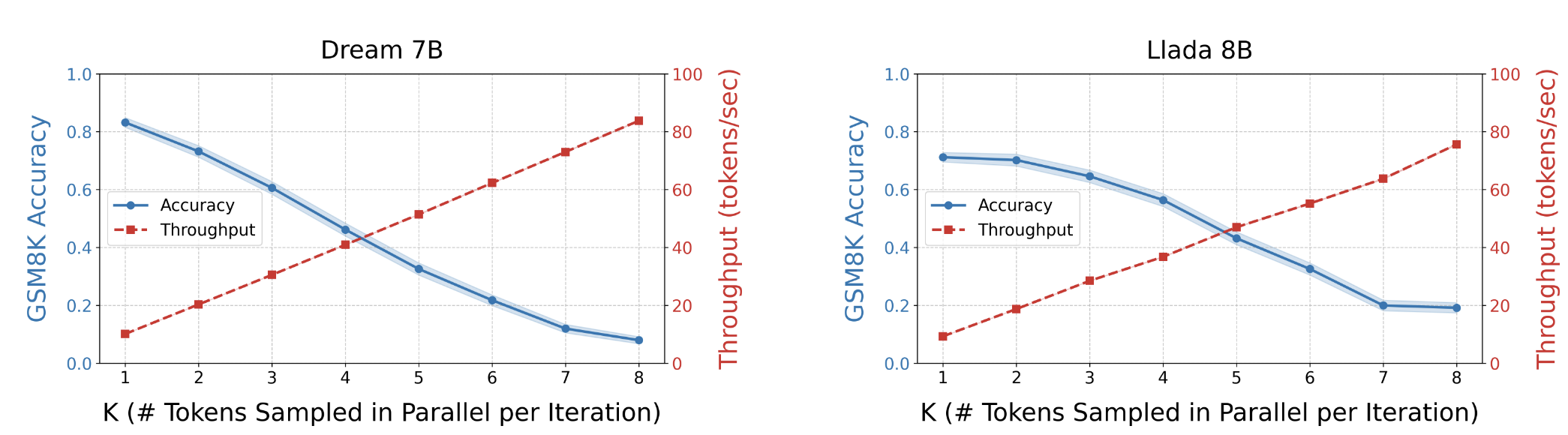 Speed vs. accuracy tradeoff on GSM8K: more parallel tokens means faster generation but lower accuracy.
On GSM8K (grade school math), accuracy drops in a very predictable manner while speed goes up. This seems fairly intuitive, but what exactly is going on? The paper Discrete Copula Diffusion16 has an excellent figure to explain this.
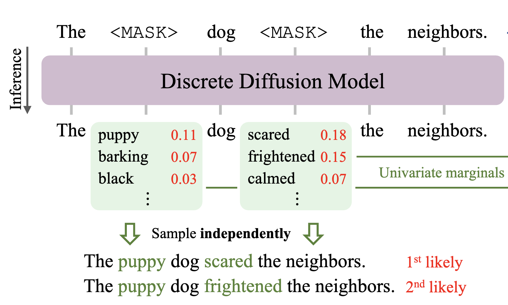 Discrete Copula Diffusion: “puppy” and “scared” are each marginally likely, but jointly unlikely.
When you sample multiple tokens in parallel, you necessarily only capture their marginal distribution. You cannot model the dependencies between them, because each token doesn’t know what the other will commit to. In this example, “puppy” and “scared” are marginally likely, but jointly unlikely. Thus, more parallelism (and speed) leads to fewer dependencies captured, and hence lower fluency.
Trading Diversity for Speed
Imagine in the example above if “barking” and “scared” had a marginal probability of 1. It would follow that their joint likelihood would also be 1, and so the product of marginal probabilities would be equivalent to the joint probability.
It turns out this logic extends to marginal probabilities near 1 as well. In fast-dLLM 17, the authors use a strategy that samples tokens at positions that exceed some probability threshold. Specifically, they state that for a joint distribution $p(x)$ and marginal product distribution $q(x)$ that factorizes $p$, if each marginal in the product has probability greater than $1 - \epsilon$, then we can bound the total variation distance between the joint and the marginal:
\[\text{TVD}(p, q) < \frac{3n-1}{2} \epsilon\]on a sequence of $n$ tokens to be sampled. For sufficiently small $\epsilon$, specifically $\epsilon \leq \frac{1}{n+1}$, this sampling method will be exactly equivalent to greedy decoding, meaning it will only sample the most likely sequence from $p$. I’m not being fully precise with the notation, and I encourage those interested to read the details, but the overall point should be clear: one can significantly improve speed at the expense of diversity.
I learned this working on Adaptive Parallel Decoding (APD)6. APD defines a multiplicative mixture between the dLLM marginals and a small autoregressive model and samples left to right from this distribution, only accepting parallel samples with high likelihood from both.
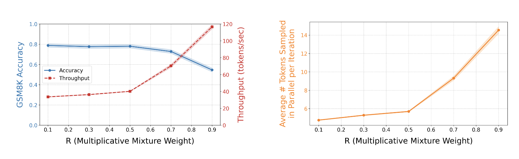 APD can dramatically increase speed with some expense to fluency and diversity.
I also introduced a parameter $R$ that controls the tradeoff. As you can see from this plot, compared to before just modifying the number of denoising steps like before, we are able to achieve a much better tradeoff. This method can improve speed by a factor of almost 10x without a significant drop in quality. It’s hard to imagine that this is free, and indeed, I think the price paid is in diversity. A multiplicative mixture between distributions inherently reduces diversity (or entropy if you prefer).
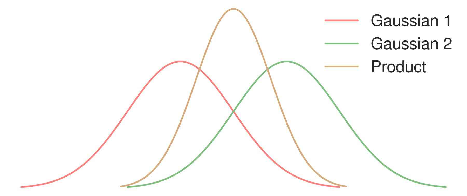 A product-of-experts18 decreases diversity
In many cases, losing diversity may be a worthy tradeoff. Does coding really need a diversity of samples? Maybe reasoning does not require diversity.
In defense of diversity
I claim that many writing tasks will require diversity, especially as we see the internet become saturated with “LLM slop” 19. Also, parallel decoding and faster inference will only lead to more intelligent models if diversity can be preserved somehow. It would be great if we could plug parallel decoding methods into modern Reinforcement Learning (RL) frameworks, because the bottleneck of RL is typically the speed of inference. However, it is widely understood that RL methods work by essentially sharpening the distribution of the LLM, revealing capabilities that have probability mass under the base model 20. Using our terminology, RL allows models to trade fluency error for diversity error (also note that they trade speed for fluency by outputting more tokens). If by parallel decoding, one removes all the diversity, then there will be almost nothing left for RL to sharpen.
No Free Lunch
Let’s revisit the claim that there is no free lunch. Is there a way to increase speed (i.e., parallel sampling) without sacrificing fluency or diversity? What about speculative decoding?
Speculative decoding 21 seems to increase parallelism at zero cost. To clarify, I believe there is no free lunch at a fixed level of compute and data. Speculative decoding uses an auxiliary draft model, which I interpret as adding more compute to the input side of the ledger. It does seem, though, that there is something profound with speculative decoding. While I maintain that parallel sampling has no free lunch, perhaps parallel verification (i.e., likelihood computation) which can be used for sampling is free. TiDAR 22 seems like a promising approach along these lines.
Instead of just adding compute to the inputs of the model, it is possible to also add data. This is what we show in Planned Diffusion7, where we train a model to use control tags to first plan a response, then use diffusion to generate from that plan to increase parallelism.
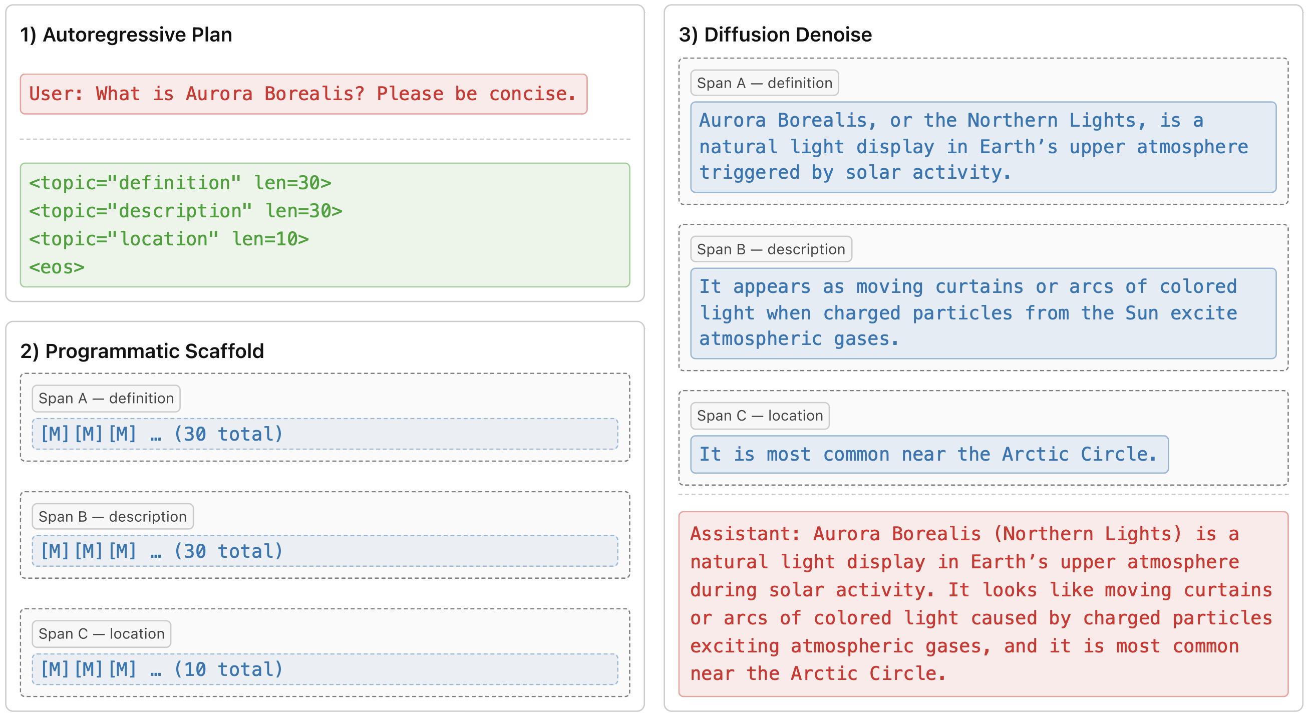 Planned Diffusion: first generate a plan autoregressively, then fill in spans in parallel with diffusion.
This type of approach is trying to improve what we call “semantic parallelism” 23. If you believe as I do that there is no free lunch with respect to speed, fluency, and diversity, adding more data seems like the best solution. After all, just adding more data until the problem was fixed is how we got LLMs in the first place 24.
Concluding Remarks
To summarize, you can add compute and data into an LLM and get out a fixed amount of speed, fluency, and diversity:
- You can trade diversity or speed for fluency through RL
- You can trade fluency for speed via fewer diffusion denoising steps
- You can trade diversity for speed with better sampling techniques
To my knowledge, I don’t know a way to trade fluency for diversity or speed—but maybe those are bad trades that are not even worth investigating.
There are now benchmarks that analyze the tradeoff between speed and quality in diffusion LLMs 25, and I encourage readers to work on algorithms to get the best tradeoffs. However, I think it is a mistake to collapse fluency and diversity into a single metric. In fact, I worry that the LLM community as a whole has over-focused on fluency, and I find it likely that more diversity is needed to push the field forward.
I look forward to novel approaches navigating the parallel decoding trilemma.
Thanks for reading! Feel free to reach out with questions or comments.
Cite This Post
@misc{israel2025trilemma,
  title        = {The Parallel Decoding Trilemma},
  author       = {Israel, Daniel},
  year         = {2025},
  month        = {November},
  howpublished = {Blog post},
  url          = {https://danielmisrael.github.io/posts/2025/11/parallel-decoding-trilemma/}
}
References
Austin, Jacob, et al. “Structured Denoising Diffusion Models in Discrete State-Spaces.” NeurIPS, 2021. arXiv:2107.03006 ↩
Lou, Aaron, Chenlin Meng, and Stefano Ermon. “Discrete Diffusion Modeling by Estimating the Ratios of the Data Distribution.” arXiv preprint, 2023. arXiv:2310.16834 ↩
Sahoo, Subham, et al. “Simple and Effective Masked Diffusion Language Models.” NeurIPS, 2024. arXiv:2406.07524 ↩
Nie, Shen, et al. “Large Language Diffusion Models.” arXiv preprint, 2025. arXiv:2502.09992 ↩
Ye, Jiacheng, et al. “Dream 7B: Diffusion Large Language Models.” arXiv preprint, 2025. arXiv:2508.15487 ↩
Daniel Israel, Guy Van den Broeck, and Aditya Grover. “Accelerating Diffusion LLMs via Adaptive Parallel Decoding.” Advances in Neural Information Processing Systems 38 (NeurIPS), 2025. arXiv:2506.00413 ↩ ↩2 ↩3
Daniel Israel, Tian Jin, Ellie Cheng, Guy Van den Broeck, Aditya Grover, Suvinay Subramanian, and Michael Carbin. “Planned Diffusion.” arXiv preprint, 2025. arXiv:2510.18087 ↩ ↩2
Jentzsch, Sophie, and Kristian Kersting. “ChatGPT is Fun, but It is Not Funny! Humor is Still Challenging Large Language Models.” arXiv preprint, 2023. arXiv:2306.04563 ↩
Sajjadi, Mehdi SM, et al. “Assessing Generative Models via Precision and Recall.” NeurIPS, 2018. arXiv:1806.00035 ↩
Xu, Ziwei, Sanjay Jain, and Mohan Kankanhalli. “Hallucination is Inevitable: An Innate Limitation of Large Language Models.” arXiv preprint, 2024. arXiv:2401.11817 ↩
Thanh-Tung, Hoang, and Truyen Tran. “Catastrophic Forgetting and Mode Collapse in GANs.” IJCNN, 2020. arXiv:1807.04015 ↩
Devlin, Jacob, et al. “BERT: Pre-training of Deep Bidirectional Transformers for Language Understanding.” NAACL, 2019. arXiv:1810.04805 ↩
Khanna, Samar, et al. “Mercury: Ultra-Fast Language Models Based on Diffusion.” arXiv preprint, 2025. arXiv:2506.17298 ↩
Shih, Andy, Dorsa Sadigh, and Stefano Ermon. “Training and Inference on Any-Order Autoregressive Models the Right Way.” NeurIPS, 2022. arXiv:2205.13554 ↩
Chandrasegaran, Keshigeyan, Armin W. Thomas, et al. “RND1: Simple, Scalable AR-to-Diffusion Conversion.” Radical Numerics, 2025. radicalnumerics.ai ↩
Liu, Anji, et al. “Discrete copula diffusion.” arXiv preprint, 2024. arXiv:2410.01949 ↩
Wu, Chengyue, et al. “Fast-dLLM: Training-Free Acceleration of Diffusion LLM by Enabling KV Cache and Parallel Decoding.” arXiv preprint, 2025. arXiv:2505.22618 ↩
Hinton, Geoffrey E. “Training Products of Experts by Minimizing Contrastive Divergence.” Neural Computation, 2002. PDF ↩
Paredes, Jose, et al. “More Articles Are Now Created by AI Than Humans.” Graphite, 2024. graphite.io ↩
Yue, Yang, et al. “Does Reinforcement Learning Really Incentivize Reasoning Capacity in LLMs Beyond the Base Model?” arXiv preprint, 2025. arXiv:2504.13837 ↩
Leviathan, Yaniv, Matan Kalman, and Yossi Matias. “Fast Inference from Transformers via Speculative Decoding.” ICML, 2023. arXiv:2211.17192 ↩
Liu, Jingyu, et al. “TiDAR: Think in Diffusion, Talk in Autoregression.” arXiv preprint, 2025. arXiv:2511.08923 ↩
Jin, Tian, et al. “Learning to Keep a Promise: Scaling Language Model Decoding Parallelism with Learned Asynchronous Decoding.” arXiv preprint, 2025. arXiv:2502.11517 ↩
Kaplan, Jared, et al. “Scaling laws for neural language models.” arXiv preprint, 2020. arXiv:2001.08361 ↩
Kang, Wonjun, et al. “ParallelBench: Understanding the Trade-offs of Parallel Decoding in Diffusion LLMs.” arXiv preprint, 2025. arXiv:2510.04767 ↩